Global Classements Analysis (all AFTT)
Source:vignettes/Vignette3_GlobalAnalysis.Rmd
Vignette3_GlobalAnalysis.RmdTo be cont’d
Analysis of current percentage of each classement
# Active players
Actifs_AFTT <- players_m[players_m[, "position_bis"] != "Inactive", ]

# Actives by classement
tab_classement_Actifs_AFTT <- table(Actifs_AFTT[, "classement"])
pct_classement_AFTT <- tab_classement_Actifs_AFTT / nrow(Actifs_AFTT)

df_class_AFTT <- data.frame(
  classement = names(tab_classement_Actifs_AFTT),
  pct_classement_AFTT = round(as.numeric(pct_classement_AFTT),digits=4)
)
noAB0<-c("NC","E6","E4","E2","E0","D6","D4","D2","D0","C6","C4","C2","C0","B6","B4","B2")
df_class_AFTT[df_class_AFTT$classement %in% noAB0,]
## classement pct_classement_AFTT
## 32 B2 0.0096
## 33 B4 0.0153
## 34 B6 0.0263
## 35 C0 0.0329
## 36 C2 0.0434
## 37 C4 0.0536
## 38 C6 0.0578
## 39 D0 0.0593
## 40 D2 0.0617
## 41 D4 0.0646
## 42 D6 0.0714
## 43 E0 0.0651
## 44 E2 0.0833
## 45 E4 0.1020
## 46 E6 0.0990
## 47 NC 0.1492
# Actives by classement letter
tab_lettre_Actifs_AFTT <- table(Actifs_AFTT[, "classement_lettre"])
pct_letter_AFTT <- tab_lettre_Actifs_AFTT / nrow(Actifs_AFTT)
pct_label_AFTT <- paste0(round(100 * pct_letter_AFTT), "%")

df_labels_AFTT <- data.frame(
  classement_lettre = names(tab_lettre_Actifs_AFTT),
  pct_letter_AFTT = as.numeric(pct_letter_AFTT),
  pct_label_AFTT = pct_label_AFTT
)
df_labels_AFTT
## classement_lettre pct_letter_AFTT pct_label_AFTT
## 1 A 0.001837919 0%
## 2 B 0.054907817 5%
## 3 C 0.187639998 19%
## 4 D 0.257021423 26%
## 5 E 0.349376831 35%
## 6 NC 0.149216013 15%Plot of the frequency of each classement for all AFTT players (actives or all)
graph.pct.classements(players_m)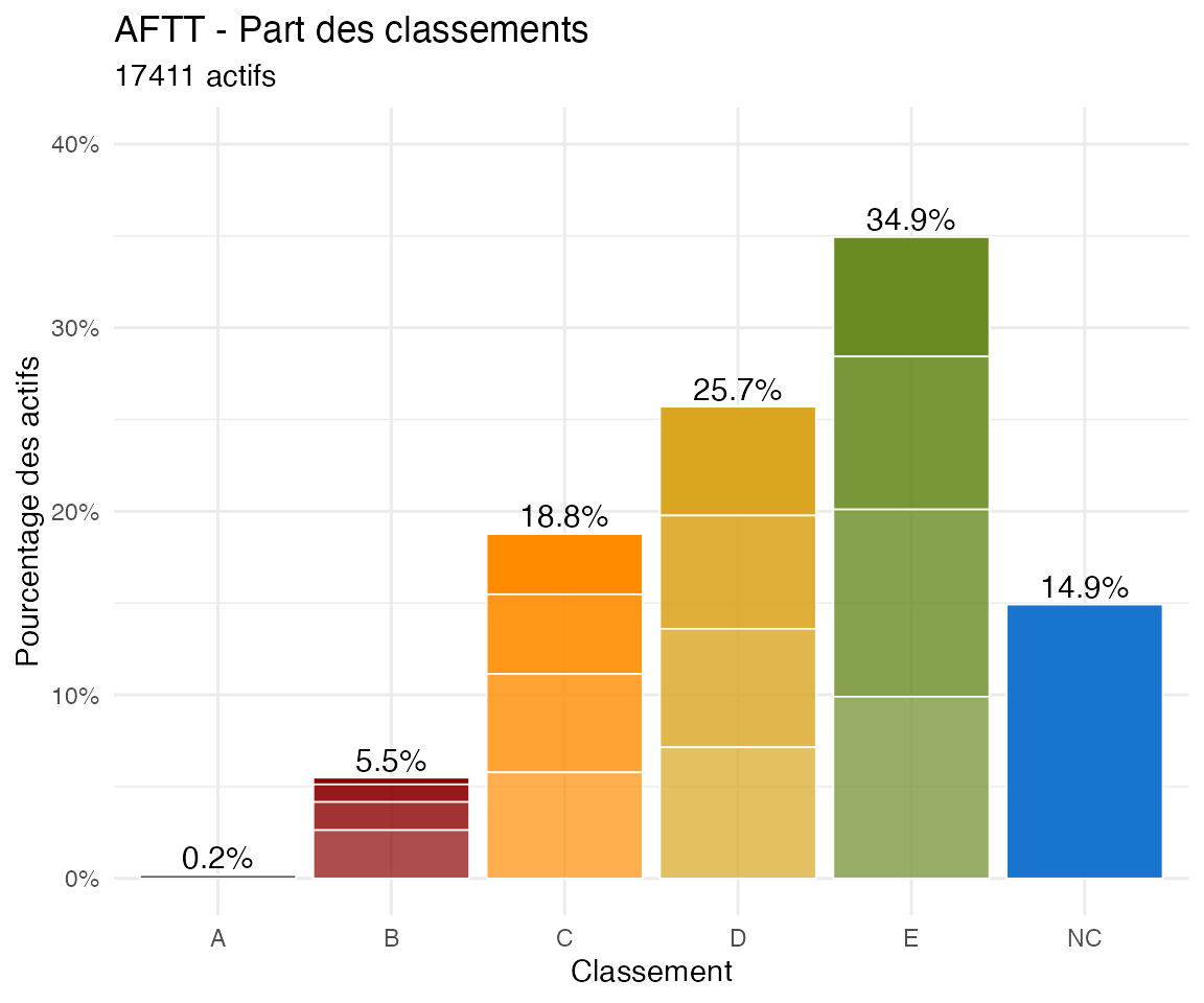
graph.pct.classements
graph.pct.classements(players_m,actifs_only = FALSE)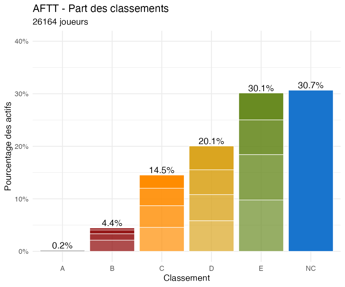
graph.pct.classements
Analysis of points per classement
players_AFTT_noA <- players_m[players_m$classement_lettre != "A", ]
players_AFTT_noA$classement <- factor(players_AFTT_noA$classement)
Points_class_qt <- aggregate(points ~ classement, data = players_AFTT_noA, FUN = quantile)
Points_class_qt <- do.call(data.frame, Points_class_qt)

Points_class_mean <- aggregate(points ~ classement, data = players_AFTT_noA, FUN = mean)
Points_class <- merge(Points_class_mean, Points_class_qt, by = "classement")
names(Points_class) <- c("classement",
                         "mean_pts",
                         "min_pts",
                         "qt25_pts",
                         "median_pts",
                         "qt75_pts",
                         "max_pts")

Points_class
## classement mean_pts min_pts qt25_pts median_pts qt75_pts max_pts
## 1 B0 2442.1399 2308.80 2338.5250 2437.385 2506.7875 2694.69
## 2 B2 2227.8380 1996.41 2161.3925 2215.800 2295.1900 2610.41
## 3 B4 2004.1629 1802.72 1941.4400 1995.000 2060.1975 2284.89
## 4 B6 1818.5295 1531.15 1759.6550 1818.670 1869.5150 2126.53
## 5 C0 1664.6280 1256.81 1602.6600 1660.350 1718.2400 1992.02
## 6 C2 1508.6019 1127.81 1452.1900 1503.390 1564.4950 1956.30
## 7 C4 1361.4511 1083.51 1304.0500 1357.720 1414.6350 1745.58
## 8 C6 1231.9200 813.76 1163.5800 1224.280 1289.4000 1637.74
## 9 D0 1100.5793 802.39 1035.6575 1088.660 1153.9475 1538.55
## 10 D2 983.4690 695.54 917.0250 973.365 1030.4825 1599.21
## 11 D4 864.0185 609.26 798.5425 854.140 914.3275 1414.12
## 12 D6 758.0462 495.36 688.6250 744.440 806.9900 1412.65
## 13 E0 638.3574 293.50 571.1975 625.640 685.7100 1274.36
## 14 E2 512.4727 192.56 438.1825 500.265 566.3500 1387.11
## 15 E4 365.7516 0.00 292.6100 343.875 421.2950 981.10
## 16 E6 209.2150 0.00 140.9125 187.000 263.6650 800.45
## 17 NC 101.8065 0.00 93.2200 100.000 100.0000 801.35
classement_cols <- c(B0 = "darkred",B2 = "darkred",B4 = "darkred",
  B6 = "darkred",C0 = "darkorange",C2 = "darkorange",
  C4 = "darkorange",C6 = "darkorange",D0 = "goldenrod",
  D2 = "goldenrod",D4 = "goldenrod",D6 = "goldenrod",
  E0 = "olivedrab4",E2 = "olivedrab4",E4 = "olivedrab4",
  E6 = "olivedrab4",NC = "dodgerblue3")

ggplot(players_AFTT_noA,
       aes(x = points,y = classement,
         fill = classement, color = classement)) +
  geom_density_ridges(scale = 2, rel_min_height = 0.01,
                      color = NA) +
  geom_vline(data = Points_class,
    aes(xintercept = mean_pts, color = classement),
    linewidth = 0.4, alpha = 0.5) +
  scale_fill_manual(values = classement_cols) +
  scale_color_manual(values = classement_cols) +
  scale_x_continuous(breaks = Points_class$mean_pts,
                     labels = round(Points_class$mean_pts, 0)) +
  theme_minimal(base_size = 14) +
  xlab("points (1er mois précédent)") +
  theme(axis.text.x = element_text(angle = 90,vjust = 0.5,
                                   hjust = 1,
                                   color = classement_cols[Points_class$classement],face = "bold"),
        legend.position = "none")
## Picking joint bandwidth of 20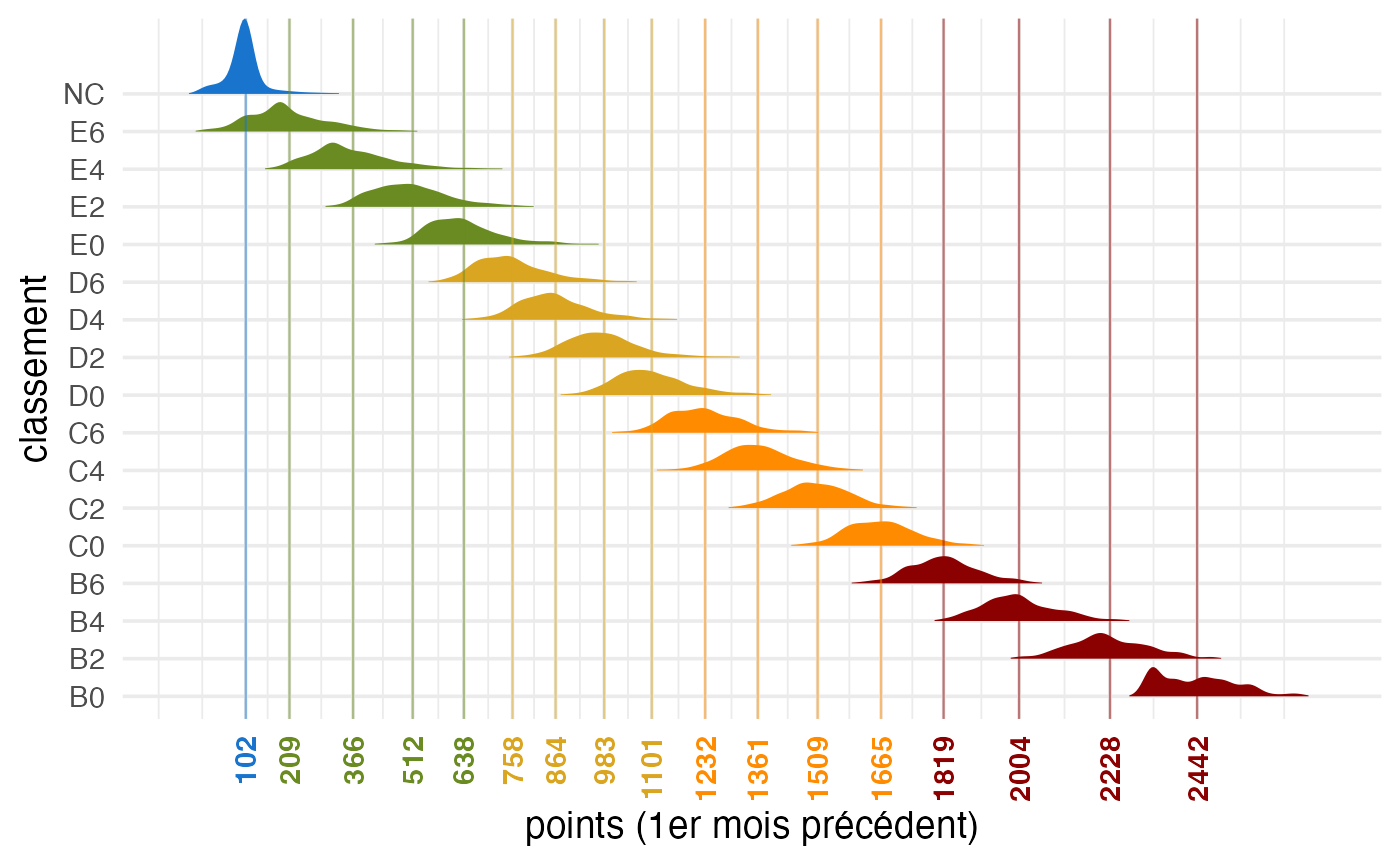
Points_class
Estimate of new classement and analysis of change
To estimate the new classement for a series of players, use the
players.new.classement() function. It is based on current
points of each players and the total number of active players retrieved
by count.actives(). The function adds 2 columns in the data
frame: the new classement (classement_new) and the number
of classements upward or downward (classement_diff). After
computing, two tables are displayed, showing - a transition table with
frequencies of players in each pair of old to new classement. Most
players (about 50%) don’t change of classement hence the diagonal is
strong. Also there are more upward changes than downward changes,
meaning training efforts generally pays-off! However you will notice
that from D4 and upper, there is usually more people going one
classement down than up. - a difference table, where we see most players
don’t change of classement and only few gain 3 or more classements in a
season. The average is around 0.3 classement, which is a rate to which
every club or province could compare as a way to measure
performance.
Applied to all players (default), the computation gives:
## [1] 17411
players_m_new <- players.new.classement()## Best guess cumulated percentage based on means across columns of the provided grille. Excludes A's and B0 players as their number is fixed##
## Transition table:
## new
## old NC E6 E4 E2 E0 D6 D4 D2 D0 C6 C4 C2 C0 B6 B4 B2
## NC 516 1755 270 50 5 1 1 . . . . . . . . .
## E6 . 851 735 120 12 5 1 . . . . . . . . .
## E4 . 75 963 606 90 28 10 4 . . . . . . . .
## E2 . 1 137 863 335 85 18 8 2 . 1 . . . . .
## E0 . . 4 195 611 226 76 18 1 2 . . . . . .
## D6 . . . 6 240 605 285 83 20 3 2 . . . . .
## D4 . . . . 22 247 553 228 61 8 5 . . . . .
## D2 . . . . . 19 255 522 216 46 12 3 1 . . .
## D0 . . . . . . 13 230 559 188 39 4 . . . .
## C6 . . . . . . 2 12 232 531 190 37 2 . . .
## C4 . . . . . . . . 17 220 535 153 9 . . .
## C2 . . . . . . . . 2 5 164 466 108 9 1 .
## C0 . . . . . . . . . 1 2 128 355 83 3 .
## B6 . . . . . . . . . . . 4 105 299 50 .
## B4 . . . . . . . . . . . . . 59 181 27
## B2 . . . . . . . . . . . . . . 35 132
## Sum 516 2682 2109 1840 1315 1216 1214 1105 1110 1004 950 795 580 450 270 159
## new
## old Sum
## NC 2598
## E6 1724
## E4 1776
## E2 1450
## E0 1133
## D6 1244
## D4 1124
## D2 1074
## D0 1033
## C6 1006
## C4 934
## C2 755
## C0 572
## B6 458
## B4 267
## B2 167
## Sum 17315##
## Difference table (number of players upward/downward by):
##
##    -3    -2    -1     0     1     2     3     4     5     6     7   Sum
##     5   105  2322  8542  5185   928   173    40    13     1     1 17315
summary(players_m_new$classement_diff)## Min. 1st Qu. Median Mean 3rd Qu. Max. NA's
## -3.0000 0.0000 0.0000 0.3033 1.0000 7.0000 8849
attr(players_m_new, which="diff_table")##
## -3 -2 -1 0 1 2 3 4 5 6 7 Sum
## 5 105 2322 8542 5185 928 173 40 13 1 1 17315
plot(attr(players_m_new, which="diff_table")[-length(attr(players_m_new, which="diff_table"))],
     main="Montées et descentes de classement",
     xlab ="Nombre de classements en plus ou moins",
     ylab ="Fréquence (nombre de joueurs)")